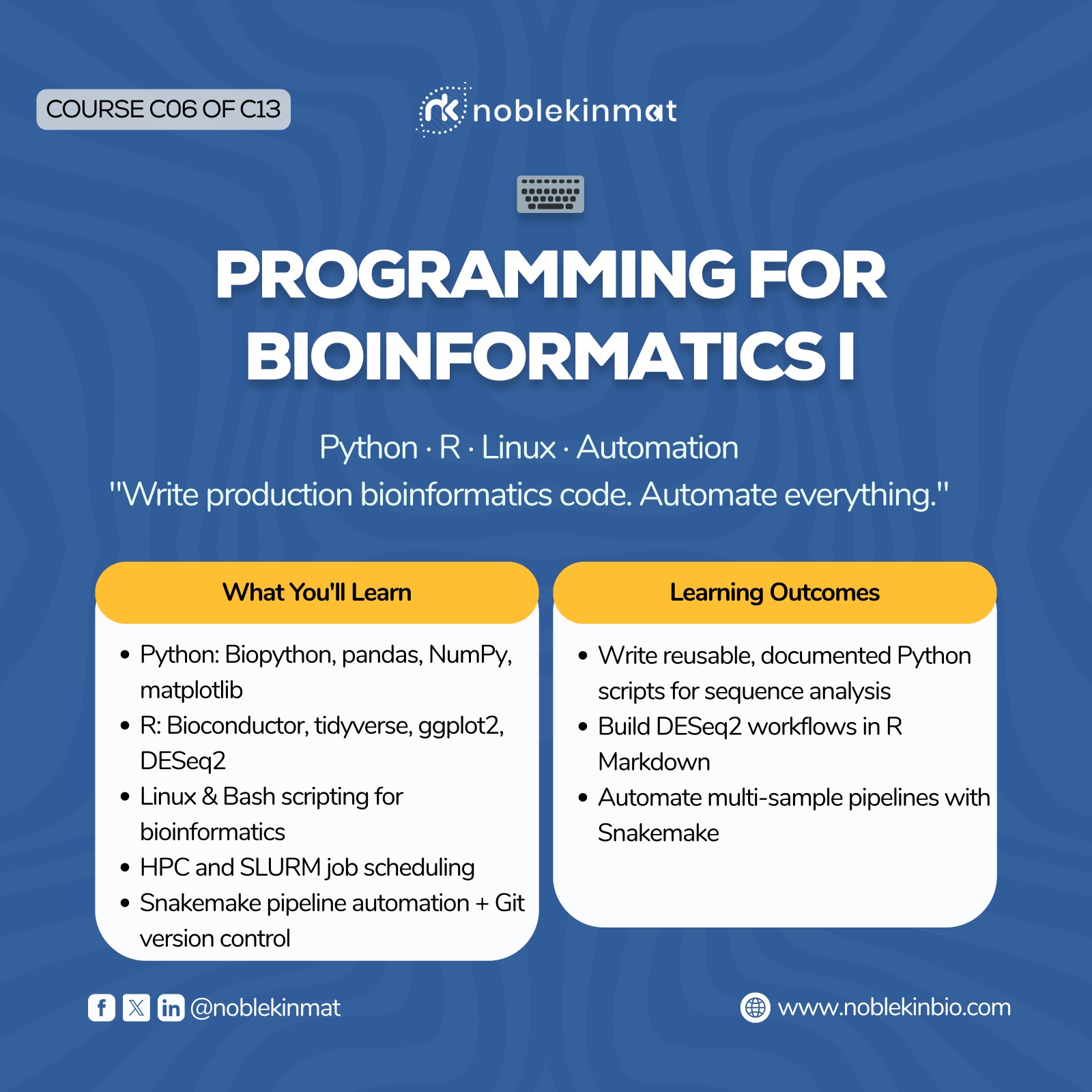
Programming for Bioinformatics I

Course Overview

This is the programming foundation course of the certificate program. Students learn Python, R, and Linux/Bash scripting specifically applied to bioinformatics problems. By the end, students write production-quality analysis pipelines that are reproducible, version-controlled, and deployable in any research environment worldwide. This course is a prerequisite for Courses 08, 09, 10, 11, and 12.

Learning Outcomes

1.     Write Python scripts to parse biological file formats, manipulate sequences, and automate NCBI queries.

2.     Use pandas and NumPy for healthcare and biological data analysis.

3.     Implement differential expression analysis pipelines in R using DESeq2 and Bioconductor.

4.     Write Bash scripts for automating multi-sample bioinformatics workflows.

5.     Build reproducible analysis pipelines using Snakemake with Conda environments.

Curriculum Content

Weeks 1–2: Python for Bioinformatics

•      Python fundamentals: data types, control flow, functions, classes, file I/O, error handling.

•      Biopython: SeqIO (FASTA/GenBank parsing), Entrez (NCBI API), BLAST (programmatic execution and parsing), pairwise2 and PairwiseAligner.

•      Data analysis: pandas DataFrames for genomic data, NumPy array operations, matplotlib/seaborn for visualisation.

•      Regular expressions: parsing biological file formats, extracting features from annotation files.

Weeks 3–4: R and Bioconductor for Bioinformatics

•      R fundamentals: vectors, data frames, lists, functions, apply family.

•      Tidyverse: dplyr (filter, mutate, group_by, summarise), ggplot2 (grammar of graphics for scientific figures).

•      Bioconductor: package installation, GenomicRanges, Biostrings, BSgenome, AnnotationDbi.

•      Statistical testing in R: t-test, Wilcoxon, chi-square, multiple testing correction (BH-FDR, Bonferroni).

•      Reproducibility with R Markdown: YAML header, code chunks, knitting to HTML/PDF.

Weeks 5–6: Linux, Bash, and Workflow Automation

•      Linux essentials: filesystem navigation, file permissions, text processing (grep, sed, awk, cut, sort, uniq).

•      Bash scripting: variables, loops, conditionals, functions, argument parsing, exit codes.

•      HPC and cluster computing: SLURM job submission, array jobs, resource allocation, module system.

•      Snakemake: rules, input/output, wildcards, params, conda directives, DAG visualisation.

•      Version control: Git — init, add, commit, push, pull, branch, merge; GitHub for collaborative bioinformatics.

Hands-On Practicals

# Python: Complete bioinformatics script — parse, analyse, report

from Bio import SeqIO, Entrez

from Bio.SeqUtils import gc_fraction

import pandas as pd, matplotlib.pyplot as plt

Entrez.email = "[email protected]"

def fetch_sequences(gene_ids):

   """Fetch multiple sequences from NCBI"""

   handle = Entrez.efetch(db="nucleotide", id=",".join(gene_ids),

                         rettype="fasta", retmode="text")

   return list(SeqIO.parse(handle, "fasta"))

def compute_stats(records):

   """Compute sequence statistics"""

   data = []

   for r in records:

       data.append({

           "id":    r.id,

           "length": len(r.seq),

           "gc":    gc_fraction(r.seq) * 100,

       })

   return pd.DataFrame(data)

# Fetch and analyse

recs = fetch_sequences(["NM_007294", "NM_000059", "NM_000546"])

df = compute_stats(recs)

print(df)

# Visualise

df.plot.bar(x="id", y="gc", color="#2ECC71", legend=False)

plt.ylabel("GC Content (%)"); plt.tight_layout(); plt.savefig("gc_content.pdf", dpi=300)

🔬 Hands-On Lab: Snakemake Pipeline for FASTQ→VCF

Step 1: Install Snakemake in a dedicated Conda environment: conda create -n snakemake -c bioconda snakemake

Step 2: Write a Snakefile with rules: fastqc → trimmomatic → bwa_mem → samtools_sort → markduplicates → haplotypecaller

Step 3: Run: snakemake --cores 4 --use-conda --dag | dot -Tsvg > workflow.svg — visualise the DAG.

Step 4: Test with two samples — use wildcards to handle arbitrary numbers of samples.

Step 5: Add a rule to produce a MultiQC report aggregating all FastQC outputs.